If Data Set A Has A Larger Mean Than Data Set B, What Would Be Different About Their Distributions?

Descriptive Statistics

12 Skewness and the Mean, Median, and Mode

Consider the following data set.
4; v; 6; 6; 6; vii; 7; 7; 7; 7; seven; 8; 8; eight; 9; x

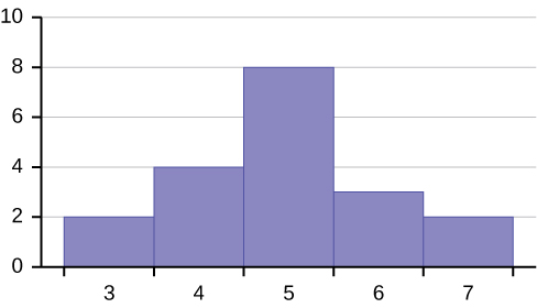
This data set can be represented by following histogram. Each interval has width one, and each value is located in the middle of an interval.

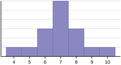
This histogram matches the supplied data. It consists of 7 adjacent bars with the x-axis split into intervals of 1 from 4 to 10. The heighs of the bars peak in the middle and taper symmetrically to the right and left.

The histogram displays a symmetrical distribution of data. A distribution is symmetrical if a vertical line can be drawn at some point in the histogram such that the shape to the left and the correct of the vertical line are mirror images of each other. The hateful, the median, and the way are each seven for these data. In a perfectly symmetrical distribution, the mean and the median are the same. This example has one mode (unimodal), and the fashion is the same as the mean and median. In a symmetrical distribution that has two modes (bimodal), the ii modes would be different from the mean and median.

The histogram for the data: 4 5 half dozen 6 6 7 7 vii vii 8 is not symmetrical. The right-manus side seems "chopped off" compared to the left side. A distribution of this type is called skewed to the left because it is pulled out to the left. Nosotros tin can formally measure out the skewness of a distribution only as nosotros can mathematically measure out the centre weight of the information or its general "speadness". The mathematical formula for skewness is: ${a}_{3}=\sum \frac{{\left({x}_{i}-\overline{x}\right)}^{3}}{n{s}^{3}}$ . The greater the divergence from zero indicates a greater degree of skewness. If the skewness is negative then the distribution is skewed left as in (Figure). A positive measure of skewness indicates right skewness such as (Figure).

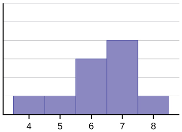
This histogram matches the supplied data. It consists of 5 adjacent bars with the x-axis split into intervals of 1 from 4 to 8. The peak is to the right, and the heights of the bars taper down to the left.

The mean is 6.3, the median is 6.v, and the style is 7. Notice that the mean is less than the median, and they are both less than the mode. The mean and the median both reflect the skewing, but the hateful reflects it more so.

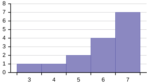
The histogram for the data: 6 7 7 7 7 8 8 viii 9 10 , is also not symmetrical. It is skewed to the right.

This histogram matches the supplied data. It consists of 5 adjacent bars with the x-axis split into intervals of 1 from 6 to 10. The peak is to the left, and the heights of the bars taper down to the right.

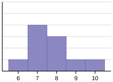
The mean is 7.7, the median is 7.5, and the mode is seven. Of the three statistics, the mean is the largest, while the mode is the smallest. Again, the mean reflects the skewing the most.

To summarize, by and large if the distribution of data is skewed to the left, the hateful is less than the median, which is ofttimes less than the way. If the distribution of information is skewed to the right, the mode is often less than the median, which is less than the hateful.

Equally with the hateful, median and mode, and as we volition see soon, the variance, there are mathematical formulas that requite u.s.a. precise measures of these characteristics of the distribution of the data. Again looking at the formula for skewness we come across that this is a relationship between the mean of the data and the individual observations cubed.

${a}_{3}=\sum \frac{{\left({x}_{i}-\overline{x}\right)}^{3}}{n{s}^{3}}$

where $s$ is the sample standard divergence of the information, ${X}_{i}$ , and $\overline{x}$ is the arithmetic mean and $n$ is the sample size.

Formally the arithmetics mean is known as the first moment of the distribution. The second moment we will see is the variance, and skewness is the 3rd moment. The variance measures the squared differences of the information from the hateful and skewness measures the cubed differences of the information from the mean. While a variance can never be a negative number, the measure of skewness tin and this is how we determine if the data are skewed correct of left. The skewness for a normal distribution is cypher, and whatever symmetric data should have skewness near zero. Negative values for the skewness indicate data that are skewed left and positive values for the skewness indicate data that are skewed right. By skewed left, we mean that the left tail is long relative to the right tail. Similarly, skewed right means that the right tail is long relative to the left tail. The skewness characterizes the degree of disproportion of a distribution effectually its mean. While the mean and standard deviation are dimensional quantities (this is why we will accept the foursquare root of the variance ) that is, have the aforementioned units as the measured quantities ${X}_{i}$ , the skewness is conventionally defined in such a way every bit to make information technology nondimensional. Information technology is a pure number that characterizes only the shape of the distribution. A positive value of skewness signifies a distribution with an asymmetric tail extending out towards more positive X and a negative value signifies a distribution whose tail extends out towards more than negative 10. A nix measure out of skewness volition indicate a symmetrical distribution.

Skewness and symmetry become important when we talk over probability distributions in after chapters.

Chapter Review

Looking at the distribution of data can reveal a lot nigh the relationship between the mean, the median, and the way. In that location are iii types of distributions. A correct (or positive) skewed distribution has a shape similar (Effigy). A left (or negative) skewed distribution has a shape like (Figure). A symmetrical distrubtion looks similar (Figure).

Formula Review

Formula for skewness: ${a}_{3}=\sum \frac{{\left({x}_{i}-\overline{x}\right)}^{3}}{n{s}^{3}}$
Formula for Coefficient of Variation: $CV=\frac{s}{\overline{x}}·100\phantom{\rule{0.2em}{0ex}}\text{conditioned upon}\phantom{\rule{0.2em}{0ex}}\overline{x}\ne 0$

Use the following information to answer the adjacent three exercises: Country whether the data are symmetrical, skewed to the left, or skewed to the right.

1 1 1 ii two 2 2 3 three 3 three 3 3 iii 3 four 4 iv 5 v

The data are symmetrical. The median is 3 and the hateful is 2.85. They are close, and the manner lies shut to the middle of the data, so the data are symmetrical.

87 87 87 87 87 88 89 89 90 91

The data are skewed correct. The median is 87.5 and the mean is 88.ii. Fifty-fifty though they are close, the manner lies to the left of the eye of the data, and there are many more instances of 87 than whatsoever other number, so the information are skewed right.

When the data are skewed left, what is the typical relationship betwixt the mean and median?

When the data are symmetrical, what is the typical relationship between the mean and median?

When the data are symmetrical, the mean and median are close or the same.

What word describes a distribution that has two modes?

Describe the shape of this distribution.

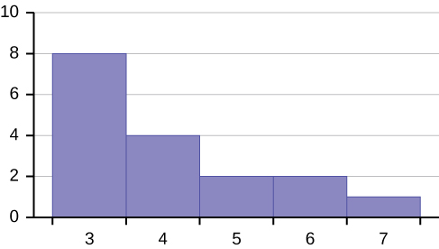
This is a historgram which consists of 5 adjacent bars with the x-axis split into intervals of 1 from 3 to 7. The bar heights peak at the first bar and taper lower to the right.

The distribution is skewed correct because it looks pulled out to the right.

Describe the human relationship between the mode and the median of this distribution.

This is a histogram which consists of 5 adjacent bars with the x-axis split into intervals of 1 from 3 to 7. The bar heights peak at the first bar and taper lower to the right. The bar ehighs from left to right are: 8, 4, 2, 2, 1.

Describe the human relationship between the mean and the median of this distribution.

This is a histogram which consists of 5 adjacent bars with the x-axis split into intervals of 1 from 3 to 7. The bar heights peak at the first bar and taper lower to the right. The bar heights from left to right are: 8, 4, 2, 2, 1.

The mean is 4.ane and is slightly greater than the median, which is 4.

Describe the shape of this distribution.

This is a histogram which consists of 5 adjacent bars with the x-axis split into intervals of 1 from 3 to 7. The bar heights peak in the middle and taper down to the right and left.

Describe the human relationship between the mode and the median of this distribution.

This is a histogram which consists of 5 adjacent bars with the x-axis split intervals of 1 from 3 to 7. The bar heights peak in the middle and taper down to the right and left.

The mode and the median are the same. In this case, they are both five.

Are the hateful and the median the exact same in this distribution? Why or why not?

This is a histogram which consists of 5 adjacent bars with the x-axis split into intervals of 1 from 3 to 7. The bar heights from left to right are: 2, 4, 8, 5, 2.

Depict the shape of this distribution.

This is a histogram which consists of 5 adjacent bars over an x-axis split into intervals of 1 from 3 to 7. The bar heights from left to right are: 1, 1, 2, 4, 7.

The distribution is skewed left because information technology looks pulled out to the left.

Describe the relationship betwixt the mode and the median of this distribution.

This is a histogram which consists of 5 adjacent bars over an x-axis split into intervals of 1 from 3 to 7. The bar heights from left to right are: 1, 1, 2, 4, 7.

Describe the human relationship between the mean and the median of this distribution.

This is a histogram which consists of 5 adjacent bars over an x-axis split into intervals of 1 from 3 to 7. The bar heights from left to right are: 1, 1, 2, 4, 7.

The hateful and the median are both six.

The mean and median for the data are the same.

3 4 5 5 vi half-dozen 6 6 7 7 7 7 seven 7 seven

Is the data perfectly symmetrical? Why or why not?

Which is the greatest, the hateful, the mode, or the median of the information set up?

11 xi 12 12 12 12 thirteen fifteen 17 22 22 22

The fashion is 12, the median is 12.v, and the mean is xv.1. The mean is the largest.

Which is the least, the mean, the fashion, and the median of the information fix?

56 56 56 58 59 60 62 64 64 65 67

Of the iii measures, which tends to reverberate skewing the most, the hateful, the mode, or the median? Why?

The hateful tends to reflect skewing the most considering it is afflicted the most by outliers.

In a perfectly symmetrical distribution, when would the mode be different from the mean and median?

Homework

The median age of the U.Southward. population in 1980 was 30.0 years. In 1991, the median historic period was 33.1 years.

What does it mean for the median historic period to rise?
Give two reasons why the median historic period could ascension.
For the median historic period to rise, is the bodily number of children less in 1991 than it was in 1980? Why or why not?